By using an RTL-SDR dongle together with a low cost noise source it is possible to measure the response of an RF filter. Also, with an additional piece of hardware called a directional coupler the standing wave ratio (SWR) of antennas can also be measured. Measuring the response of a filter can be very useful for those designing their own, or for those who just want to check the performance and characteristics of a filter they have purchased. The SWR of an antenna determines where the antenna is resonant and is important for tuning it for the frequency you are interested in listening to.
These tutorials are based heavily on information learned from Adam Alicajic’s (9A4QV), videos which can be found at [1], [2], [3], [4]. Adam is the creator of the LNA4ALL and several other RTL-SDR compatible products. Recently Tim Havens also posted some experiments with characterizing home made filters on his blog.
Characterizing Filters
Using just a noise source and RTL-SDR dongle it is possible to determine the properties of an RF filter.
In our experiments we used the following equipment:
Equipment
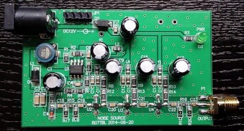
- BG7TBL Noise Source ($29.50 USD)
- 12V Power Supply that can supply at least 0.2A for powering the noise source (~$5 USD)
- RTL-SDR Dongle (~$10-$25 USD)
- T-Junction SMA Coax Splitter for testing coax stub notch filters ($2 USD)
The BG7TBL noise source is a wideband noise source that can provide strong noise over the entire frequency range of the RTL-SDR. It requires power from a 12V source which can be obtained from a common plug in power supply. It also uses an SMA female connector, so you may need some adapters to connect it to your filter under test (adapters can be found cheaply on Ebay). Finally a quick warning: be careful when handling the circuit board after it has been powered for some time as some of the components can get very hot.
If you have a ham-it-up upconverter and are good at soldering small surface mount components you might instead consider purchasing the noise source kit add on. Here is a video showing how to build and test the noise source.
Software
The software we use is as follows:
- rtl_power (keenerds build)
- RTL-SDR Panorama (or any other rtl_power GUI or RTL-SDR spectrum analyzer) – (Optional)
We will use rtl_power with the RTL-SDR Panorama GUI to record and graph a frequency sweep over the effective range of the filter. If you are experienced with command line use of rtl_power you may also use it without the GUI.
To set up RTL-SDR Panorama place the rtlpan.exe file into the same folder as rtl_power, which can be obtained from the official RTL-SDR release, or from one of keenerds builds (GitHub for Linux). We recommend using keenerds builds as his modified drivers seem to retune much faster making scans of large bandwidths significantly faster.
Characterizing Filters Tutorial
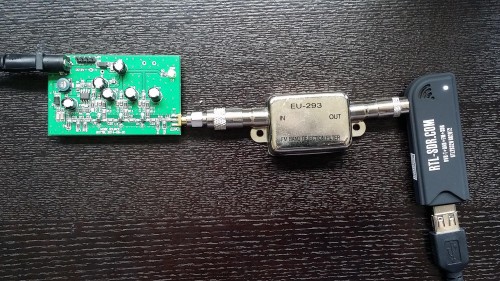
To characterize a filter simply connect the noise source to the input of the filter and the RTL-SDR to the output. Then open RTL-SDR Panorama and set the frequency range to the expected range of the filter and set the resolution to 1M. Also set the gain to 0 and enable Auto dB. Next click start and after a few seconds a graph of your filter response should be generated.
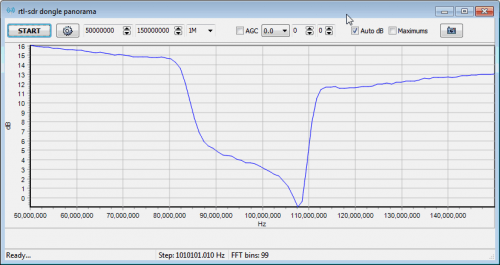
The image below shows the response of a cheap FM bandstop filter, such as the one available from MCM electronics plotted between 50 MHz and 150 MHz.
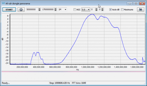
The image below shows the response of a 1090 MHz bandpass filter plotted between 100 MHz and 1.7 GHz
After viewing the response in RTL-SDR Panorama we recommend plotting the same graph against a baseline graph of just the noise source connected directly to the RTL-SDR. This can be done using Excel or any other similar plotting software. Each time RTL-SDR Panorama finishes a frequency sweep, the data is stored in a CSV file called scan.csv. It will be located in the same folder as rtlpan.exe.
First do a baseline sweep with no filters connected and then stop RTL-SDR Panorama by pressing the stop button. Note that after you press the stop button the final sweep will still be running, so wait until it finishes first. Next rename scan.csv to baseline.csv.
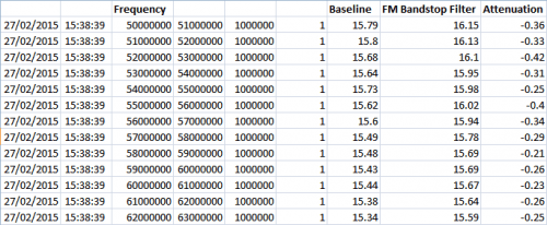
Now do a sweep with the filter connected – this will create a new scan.csv file. Next open baseline.csv in Excel. You should notice that the third column C contains the frequency values and the last column G contains the power data.
Use the excel plotting tools to create a scatter plot in baseline.csv with frequency on the x-axis and power on the y-axis. Finally, open the scan.csv which contains data for the scan with the filter. Copy the last column containing the power values (column G), and paste it into baseline.csv next to the baseline power values. Add a plot of the filtered power values to the same plot as the baseline plot and compare.
Next you can calculate the attenuation by simply subtracting the baseline column from the filter power column.
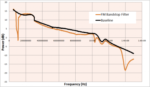
The plotted graph below shows the difference between the baseline plot (no filter connected) and the FM bandstop filter plot. There is a clear dip in power in the FM band at 88 – 108 MHz. There is also another dip at around 1.4 GHz, and some slight loss over the rest of the band due to the filter or possibly due to the type of connectors used.
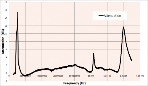
This next plot shows the attenuation, which is simply the baseline plot subtracted from the FM bandstop filter plot. The attenuation shows how strongly a signal at a particular frequency will be reduced in strength. In the graph we can see that the FM band has an attenuation of around 10 – 15 dB.
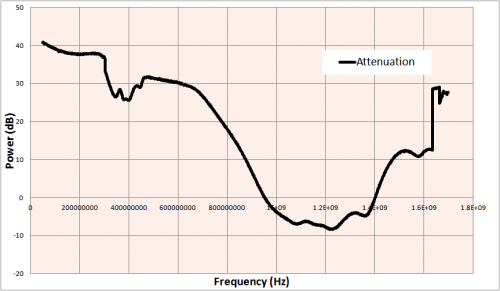
Below we also show the attenuation of the 1090 MHz ADS-B bandpass filter.
Characterizing Coax Notch/Stub Filters
Another class of filters that can be tested with a noise source and RTL-SDR are coax notch filters, aka coax stub filters. Coax stub filters are simply a length of coax, cut to 1/4 wavelength * velocity factor of the desired notch frequency. The required length can be calculated using a calculator, or by using the equation:
When cutting the coax we recommend cutting the coax a little longer and then using the noise source and RTL-SDR to fine tune the length.
The velocity factor is a parameter that is unique to each brand and type of coax cable. If you are unsure what the velocity factor is, we recommend either using the calculator (it has pre-set velocity factor values for various coax types) or determining it through the instructions shown in next heading.
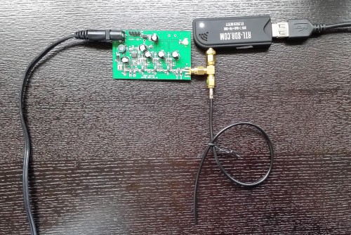
To test these filters you will need a T-junction (3-way) coax splitter. In this experiment we used a 3-way splitter with SMA connectors and used RG174U cabling with unknown velocity factor to create the coax stub filter.
The excel plot below shows the response of a coax notch filter tuned for a notch at 157 MHz, in order to attenuate strong pager signals. The plot shows that at 157 MHz there is a deep notch as expected. Note that there are also notches present at higher frequencies as well and that the notches can have quite wide bandwidths. This is expected and a potential flaw of coax stub filters.


Determining the Velocity Factor of Coax
Working backwards from the coax stub formula is it possible to determine the velocity factor of an unknown piece of coax. Simply create a coax stub filter of any known length with your suspect coax, then use the above method to measure where the main notch lies. Then use the equation:
In the previous experiment our coax stub measured 30.8 cm and had a main notch at 157 MHz. So we have a velocity factor given by the following calculation.
VF = 157 * 0.308 / 75= 0.645
This is quite close to the expected velocity factor value for most brands of RG174U which is 0.66.
Determining the VSWR of an Antenna
Equipment
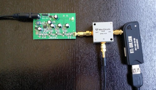
As well as the equipment needed for characterizing filters, for determining VSWR you will also need a directional coupler such as the
- MiniCircuits ZFDC-20-5 Directional Coupler (~$38 USD)
MiniCircuits directional couplers can often be found used, but in good condition on Ebay for about half price. In our experiments we actually used a MiniCircuits ZFDC-15-5 coupler with SMA connectors, but they have currently all sold out on Ebay. The ZFDC-20-5 should work just as well however. Try and find a directional coupler that works over the frequencies that you are interested in. A good video showing use of a directional coupler in a similar experiment and explaining a bit about how one works can be found here.
Determining the VSWR of an Antenna Tutorial
To measure the VSWR of an antenna we will use the directional coupler in reverse. Here we connect the noise source to the output of the coupler, the antenna to the input of the coupler and the RTL-SDR dongle to the coupling (CPL) port of the coupler. This way power from the noise source should be reflected from the antenna into the RTL-SDR.
Open the RTL-SDR Panorama GUI and enter the frequency range of which you’d like to check the VSWR of the antenna. Also, set the resolution to 1M and gain to 0.
First do a sweep with the antenna disconnected from the coupler. After the sweep is done, stop RTL-SDR Panorama and rename the scan.csv file found in the same folder as rtlpan.exe to swr.csv. Note that after clicking on stop in RTL-SDR Panorama you will need to wait for the current sweep to stop before you can rename the csv file.
Secondly do the same sweep but with the antenna connected. Now open the swr.csv file and the latest scan.csv files in Excel or any similar program and copy the power data (the last column) from scan.csv into an empty column in swr.csv.
Now subtract the values in the first power column (power with antenna disconnected) from the values in the second power column (power with antenna connected) that you have just copied over. This will give you the return loss. If you get any negative values in the return loss column you may need to adjust the values so that the negative values are forced to be a small positive value like 0.0001. In Excel this can be done using the max function such as “=max(0.0001, J2)”.
The VSWR can then be calculated from the return loss (RL) with the following equation.

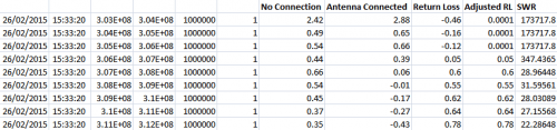
Calculate the VSWR in another column. The image below shows what your completed Excel sheet might look like.
Now plot the SWR using a scatter plot with frequency on the x-axis (horizontal) and SWR on the y-axis (vertical). Change the vertical axis to a logarithmic scale for a better view.
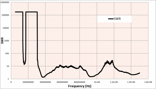
Below we show the SWR plot of a monopole antenna that is 23 cm long placed on a 20 cm diameter cookie tin that is acting as a ground plane. A perfect ground plane antenna with a 23 cm long whip should be resonant at about 310 MHz. However, because the ground plane for this antenna is only 20 cm, the SWR minimum point is pushed up to around 355 MHz. At the minimum point the SWR is about 1.15. Using a larger cookie tin would cause the minimum SWR point to approach 310 MHz.
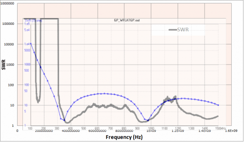
Here we compare our results with a SWR simulation of our 23 cm monopole antenna and 20 cm ground plane made in 4NEC2. We can see that the real world SWR plot approximately matches the simulation. Unmodelled factors such as coax cable and connectors used can explain some of the discrepancies.
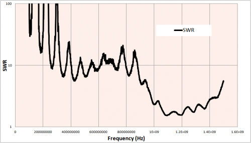
Below we show the SWR plot of a tuned 1090 MHz antenna made for ADS-B reception. The SWR at 1090 MHz is about 1.5.
Many people incorrectly believe that the SWR value does not matter for receive only antennas. This misconception probably comes from the fact that a poor SWR value on a transmitting antenna could destroy the transmitter, but a poor SWR value on a receiving antenna poses no such threat. However, while it won’t destroy your radio, a poor SWR value will still significantly impact reception. By using the calculator available at http://www.csgnetwork.com/vswrlosscalc.html, it is possible to determine the amount of signal loss you can expect with a particular SWR value. At a SWR of 1.5 we can expect a very small loss of about 0.177 dB (4% of the received power), whilst an SWR value of 10 gives a 4.807 dB loss (67% of the received power).
The post RTL-SDR Tutorial: Measuring filter characteristics and antenna VSWR with an RTL-SDR and noise source appeared first on rtl-sdr.com.